seedlookout
A Minecraft seed experience index can help answer a practical question: how much different terrain and how many kinds of destinations does this seed offer within the area I want to explore?
Our seed experience calculator calls this the Overworld Discovery Index. It combines sampled biome families and predicted structure types into a score from 0 to 100, with more credit for discoveries closer to estimated spawn. You choose the edition, generation version and radius. The score describes modeled variety; your preferences still decide whether you want to play there.
We examined 1,024 pseudorandom seeds in each of two generation models. At a 2,048-block radius, the median displayed index was 62 in Java 26.3 and 63 in Bedrock 26.50. The rubric’s mathematical ceiling of 100 is a different quantity from the center of that sample. The plots below show how to put a score in context without turning it into an enjoyment rating.
Choose an exploration radius
The calculator offers radii of 512, 1,024, 2,048 and 4,096 blocks. Each is a circle measured horizontally from estimated world spawn. A 2,048-block radius reaches that far in every direction; it does not mean a 2,048-block walk visits everything inside it.
We use 2,048 blocks as the default because the tool needs a starting area. We have not calibrated that choice against a representative measure of how far Minecraft players explore. Mojang’s exploration guide describes both short trips and larger adventures, without supplying an average radius.
Choose the radius that fits the world you want. A small circle asks about nearby variety. A larger circle includes more potential destinations and gives the same nearby discovery more distance credit. Compare two seeds at the same radius so the question stays consistent.
Radius therefore changes two things: the area searched and the credit for a particular distance. A prediction 1,024 blocks from spawn earns 0.75 credit at a radius of 2,048, but 0.875 at a radius of 4,096. A score can rise at the larger radius even before another type is found. That increase answers a broader exploration question; it does not establish that the seed itself has improved.
Count different experiences
Raw biome counts can give several points to closely related terrain. The calculator keeps those raw IDs visible, but groups related variants for scoring. Plains and sunflower plains share a family. Ocean and deep ocean share another. Flower forest has its own family; the cave families also count separately.
These families are our editorial definitions. The tool does not score advancement completion. Every eligible family has the same weight within the biome part of the score. A family is eligible only when the selected generation model’s version catalogue contains a member of it.
For surface terrain, the calculator samples a 32-block grid at approximate surface height. If that height returns a cave biome, it excludes the sample from the surface count. Narrow patches can fall between grid points, so the raw count is the number of biome IDs sampled, not an exhaustive inventory.
Cave sampling uses a 64-block grid at Y -48, -32, -16, 0, 16, 32 and 48, keeping points at least eight blocks below the approximate surface. Those samples identify cave-biome regions. A sample can lie inside solid terrain, so it does not prove there is an accessible cave at those coordinates. Vertical travel and digging effort receive no distance penalty in this first rubric.
Structures contribute by type: villages count once, regardless of how many village predictions lie inside the circle. A village and a shipwreck add two different types. The calculator searches for the nearest prediction of every eligible type, including underground destinations when its version criteria support them.
Mineshafts are excluded from every profile because the available nearest finder cannot establish coverage at all the offered radii. The score therefore measures its listed criteria, not every possible Overworld destination.
Give nearby discoveries more credit
For each found family or structure type, horizontal distance determines its credit:
credit = 1 − 0.5 × distance / radius
A discovery at spawn earns 1. At half the radius it earns 0.75, and at the boundary it earns 0.5. A criterion not found earns 0. Each category average includes every eligible criterion in its denominator, including those not found.
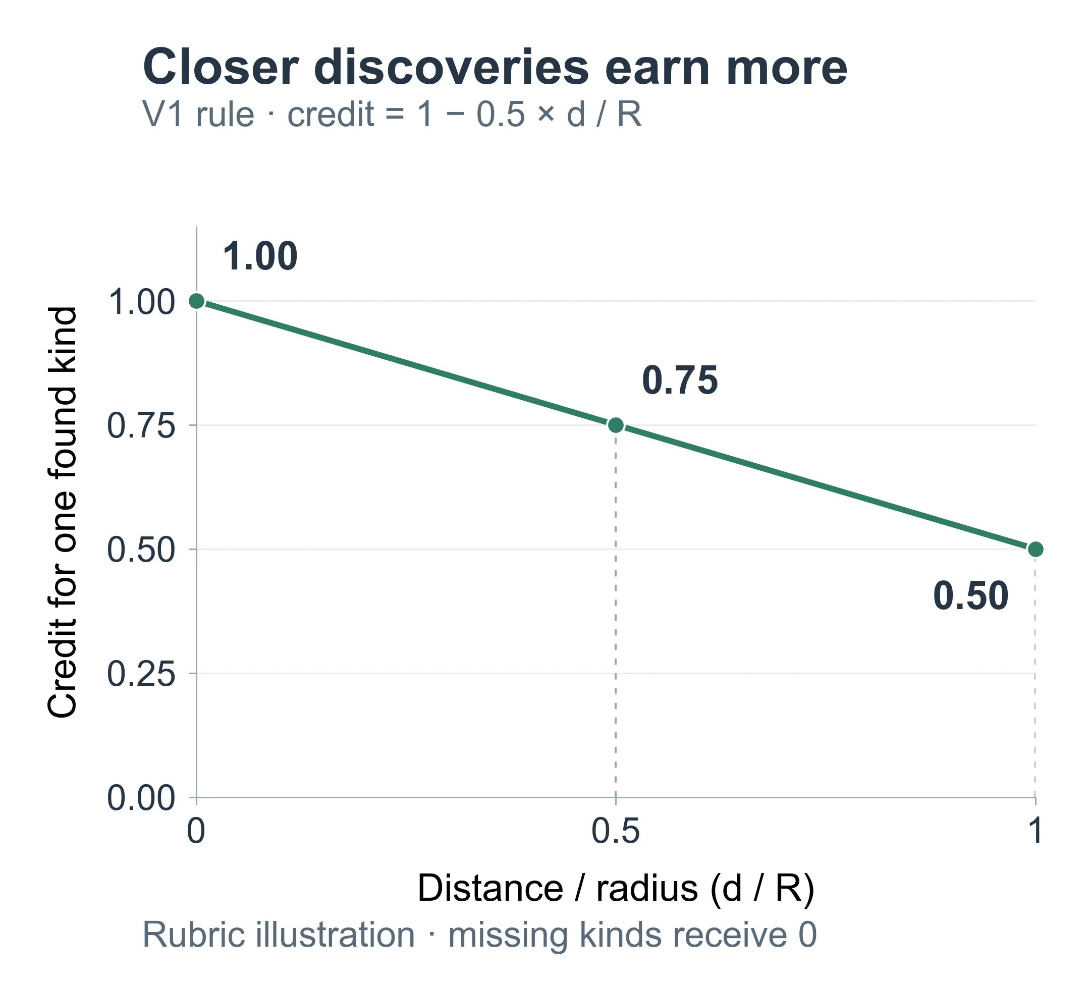
Rubric illustration, not a sample of worlds. The horizontal axis divides distance by the chosen radius; the vertical axis shows credit for one found criterion.
The final calculation gives equal weight to the two categories:
index = round(100 × (0.5 × biome average + 0.5 × structure average))
In the Java 26.3 and Bedrock 26.50 profiles, biomes can earn up to 50 points across 35 families, while structures can earn up to 50 across 17 types. One family can contribute about 50 / 35 = 1.43 index points before rounding; one structure type can contribute about 50 / 17 = 2.94. Both contributions shrink with distance. Combining all 52 criteria into a single equally weighted list would give biomes more influence; the two halves keep their total weights equal.
Here is a hypothetical example to show the arithmetic, not a result for a particular seed:
| Category | Credits across its eligible criteria | Average |
|---|---|---|
| Four biome families | 1, 0.75, 0.5, 0 | 0.5625 |
| Three structure types | 0.75, 0, 0 | 0.25 |
The index is round(100 × (0.5 × 0.5625 + 0.5 × 0.25)) = 41.
The grouping, equal category weights and half credit at the boundary are choices in revision 1. We have not fitted those choices to a survey of what players enjoy. A family or structure type does not automatically earn extra credit because it appears less often in the reference sample.
The tool also distinguishes a completed search with no prediction from an incomplete search. When bounded structure coverage leaves a type unknown, the overall score is withheld. Unknown coverage contributes neither a successful discovery nor a missing type.
Share the calculation code, review criteria by version
Minecraft version support needs two separate decisions: which generation model to use, and which calculation criteria apply.
The calculator shares one sampling and scoring core. Java and Bedrock use the site’s existing edition-specific generation models. An explicit registry connects each supported generation version to its calculation criteria. Versions can share a criteria recipe when the rules are the same; they do not need separate copies of the calculator engine.
The criteria control eligible structure types, sampling spacing, cave depths, category weights and distance credit. The biome catalogue comes from the selected model version and is matched against the reviewed family definitions. An unknown biome name or unsupported version stops the calculation until its criteria have been reviewed.
For example, the current Java 1.18.2 profile has 29 eligible biome families and 13 structure types. Java 26.3 has 35 families and 17 types. Those are calculator denominators, not counts for any individual seed. The older profile is never charged for categories outside its version’s model and criteria.
Each result identifies its edition, generation version and calculation revision. If grouping or weights change, the rubric needs a new revision. The matching reference sample must also be evaluated under those rules. This keeps the calculation maintainable while preserving the meaning of a saved result.
Read the result as a set of predictions
The result presents a large score, distance-credit bars and icons for every eligible biome family and structure type. Dim biome icons mean “not sampled”; dim structure icons mean “no prediction found.” Unknown coverage has its own state, and excluded or version-ineligible types sit outside the scored lists.
The icon collections answer which kinds were represented. The contribution bars explain how much of their possible credit survived the distance deduction. Two seeds can have the same family and type counts but different scores if their nearest discoveries lie at different distances. Keep the counts and both category contributions alongside the overall number when comparing them.
The result retains sampled surface and cave biome counts, both denominators and nearest coordinates. Its seed map links let you inspect those locations. A biome coordinate is the nearest sampled point, not an exact biome boundary. Spawn and surface height are estimates.
Structure predictions use the available placement and biome checks; later generation can still prevent a structure. Bedrock uses a compatibility model whose accuracy has not been independently checked in game. The About page explains the site’s evidence labels.
The profile covers default generation. Custom data packs, Large Biomes, superflat worlds and existing chunks generated before a world upgrade are outside its scope. Use the version that generated the area you are evaluating.
A high index does not establish attractive scenery, easy survival or valuable loot. It also does not tell you what fraction of the circle you will actually visit. An island world with a low variety score might suit you better than a seed with many nearby categories.
Calculate a seed you care about
Open the calculator, enter a seed and choose its edition and generation version. Java also accepts seed text and resolves it to a numeric seed; Bedrock takes a numeric seed. Pick a radius, then calculate.
Inspect the category breakdown before comparing the final numbers. If a particular biome or structure matters most to you, use the seed finder to search for that condition, then evaluate the surrounding variety with the calculator. The calculator’s URL retains your input settings so you can return to the same question.
What random seeds tell us
We selected 1,024 pseudorandom signed 64-bit numeric seeds and evaluated every seed in both Java 26.3 and Bedrock 26.50. Both cohorts use default Overworld generation, a 2,048-block radius and calculation revision 1, with 35 eligible biome families and 17 structure types. The same seed numbers form a paired study; each edition’s distribution is summarized separately. All 2,048 model evaluations completed, with no failed or incomplete result omitted or replaced.
We selected numeric seeds without curating them from the published catalogue. This study describes the calculator under those settings; it does not measure worlds that players chose to keep.
Read the overall distribution
The table describes the displayed, rounded index. P10 to P90 gives the sample’s 10th and 90th percentile values. Integer ties mean that the proportion between those values can exceed 80%; the range is not a confidence interval.
| Generation model | Mean index | Median index | P10 to P90 | Median families sampled | Median types predicted |
|---|---|---|---|---|---|
| Java 26.3 | 62.4 | 62 | 56 to 68 | 27 of 35 | 13 of 17 |
| Bedrock 26.50 | 62.8 | 63 | 57 to 69 | 27 of 35 | 13 of 17 |
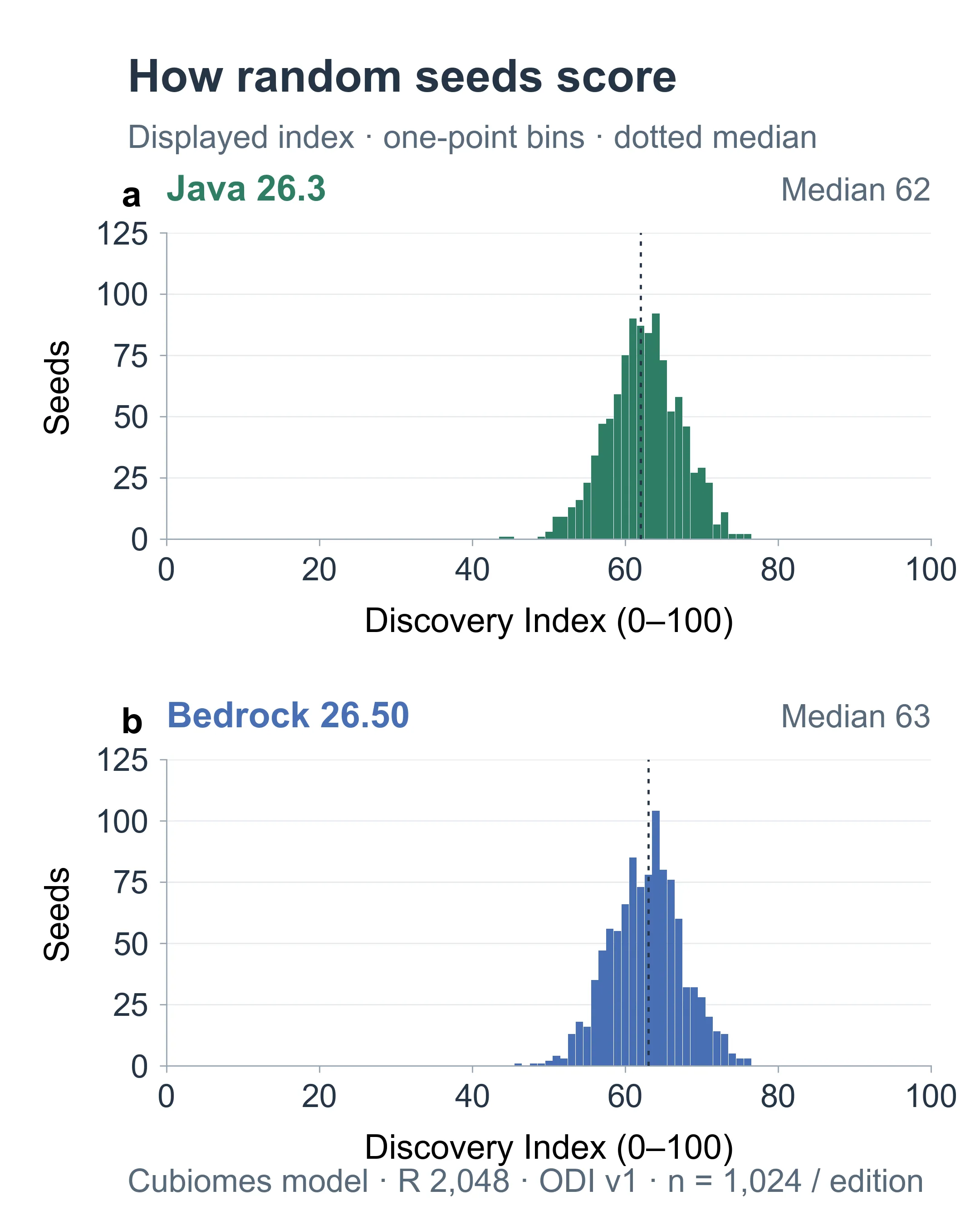
Calculator model predictions. Each narrow bar counts seeds at one displayed index value. Both panels use the full 0 to 100 score scale and the same seed-count scale.
The horizontal axis is the displayed index; the vertical axis is the number of sampled seeds receiving it. Taller bars mark more common scores in the cohort. The Java scores span 44 to 76, and the Bedrock scores span 46 to 76. Their medians sit near the middle of those observed distributions, far below the theoretical ceiling of 100.
A score of 69 is therefore above the median for either of these matching reference samples. The biome and structure breakdown explains which discoveries supplied those points.
Separate breadth from distance credit
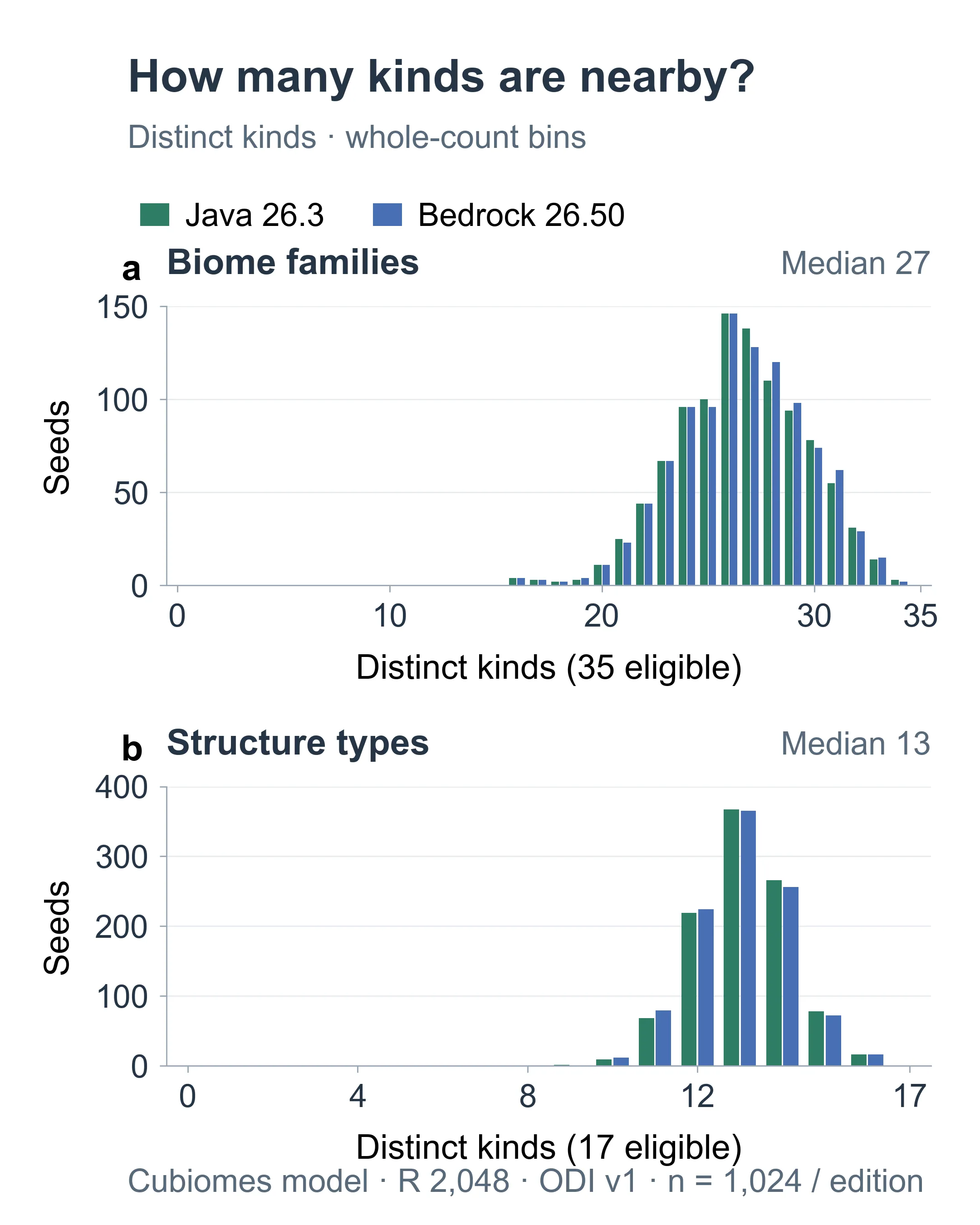
Each bar counts model seeds with a particular number of represented families or structure types. Surface and cave families are included. These counts have no distance weighting.
The upper panel asks how many different biome families were sampled inside the circle. The lower panel asks how many different structure types had a prediction inside it. Read the green and blue bars separately within each whole-number group; adding them would combine two editions whose reference settings must remain distinct.
Both editions have a median of 27 sampled families and 13 predicted types. Family counts range from 16 to 34 in each cohort. Predicted type counts range from 9 to 16 in Java and 10 to 16 in Bedrock. No sampled world represented all 35 families or all 17 types under these model settings.
Breadth answers how many kinds are represented, regardless of how far away their nearest samples or predictions are. The final score also rewards proximity. This is why neither a family count of 27 nor a structure count of 13 should be read as a component score of 27 or 13 out of 100.
Inspect the biome half
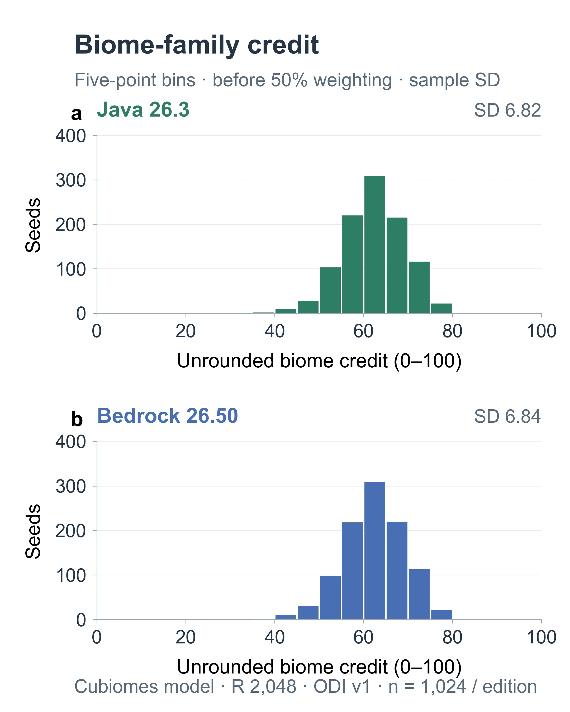
Model predictions from the same paired seed sample. These horizontal-axis values are biome scores before their half weight in the overall index.
Each bar covers a five-point interval, unlike the one-integer bars in the overall-score histogram. A biome component of 70 would contribute 35 index points before final rounding. It means that the average credit across eligible families is 0.70; it does not mean 70 families or 70% of the circle has been explored.
The biome distributions vary more widely across these samples than the structure distributions below. Their sample standard deviations are about 6.82 points in Java and 6.84 in Bedrock. NIST describes standard deviation as a measure of spread around the sample mean, expressed in the original units. Here those units are component-score points. It describes variation among seed scores, not a margin of error for the mean. Both biome distributions also show a statistically detectable departure from a normal shape in our diagnostic test after correction for multiple tests.
The family count and the distances jointly produce this spread. The histogram cannot identify which family a particular seed lacks; the calculator’s icons and coordinate details answer that question.
Inspect the structure half
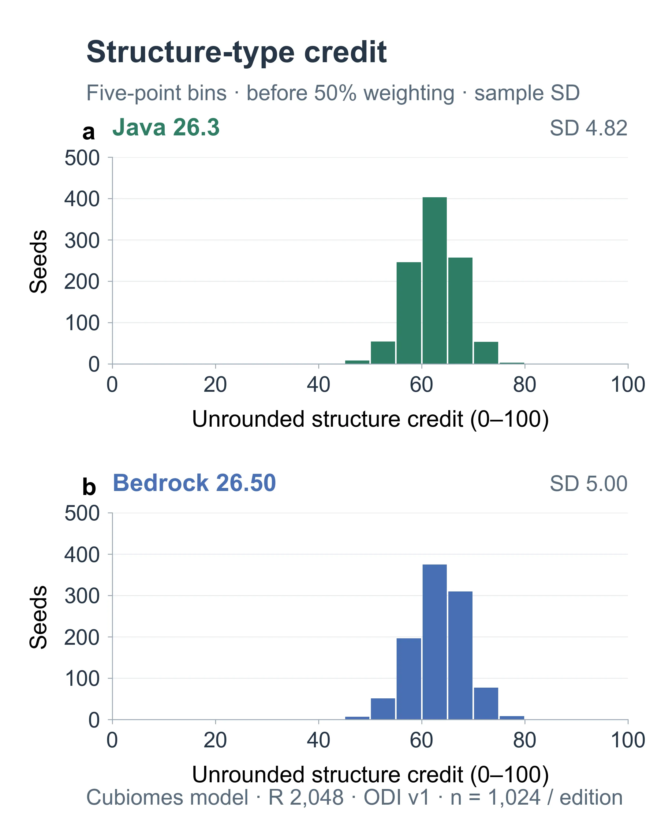
Each modeled structure type contributes once through its nearest prediction. The graph does not count all the structures in a world.
The axes and five-point bins use the same meanings as the biome-component graph, so their horizontal spreads are comparable. Each graph has its own vertical seed-count ticks. Sample standard deviations are about 4.82 points for Java and 5.00 for Bedrock, smaller than the biome component’s spread. Our corrected normality test did not reject either structure-component distribution.
The structure half combines represented type counts with horizontal proximity. Extra villages of the same type do not add variety points, and a nearby predicted stronghold receives no additional allowance for the work of reaching it underground. Those are properties of this rubric, not findings about the difficulty of those worlds.
The overall index averages these two different component scores before rounding. Its distribution can differ from either half. In these cohorts the aggregate looks approximately bell-shaped even though the biome component departs from normality. We assess that aggregate directly; combining two scores does not establish a general rule about every version or radius.
Check the tails with a normal Q-Q plot
A histogram is useful for seeing where most scores fall, but its bins can hide smaller differences in shape. The normal Q-Q plot compares the ordered unrounded scores with the scores expected from a normal distribution using each cohort’s observed mean and sample standard deviation. NIST’s explanation of normal probability plots describes how departures from a straight reference line expose differences from a normal shape.
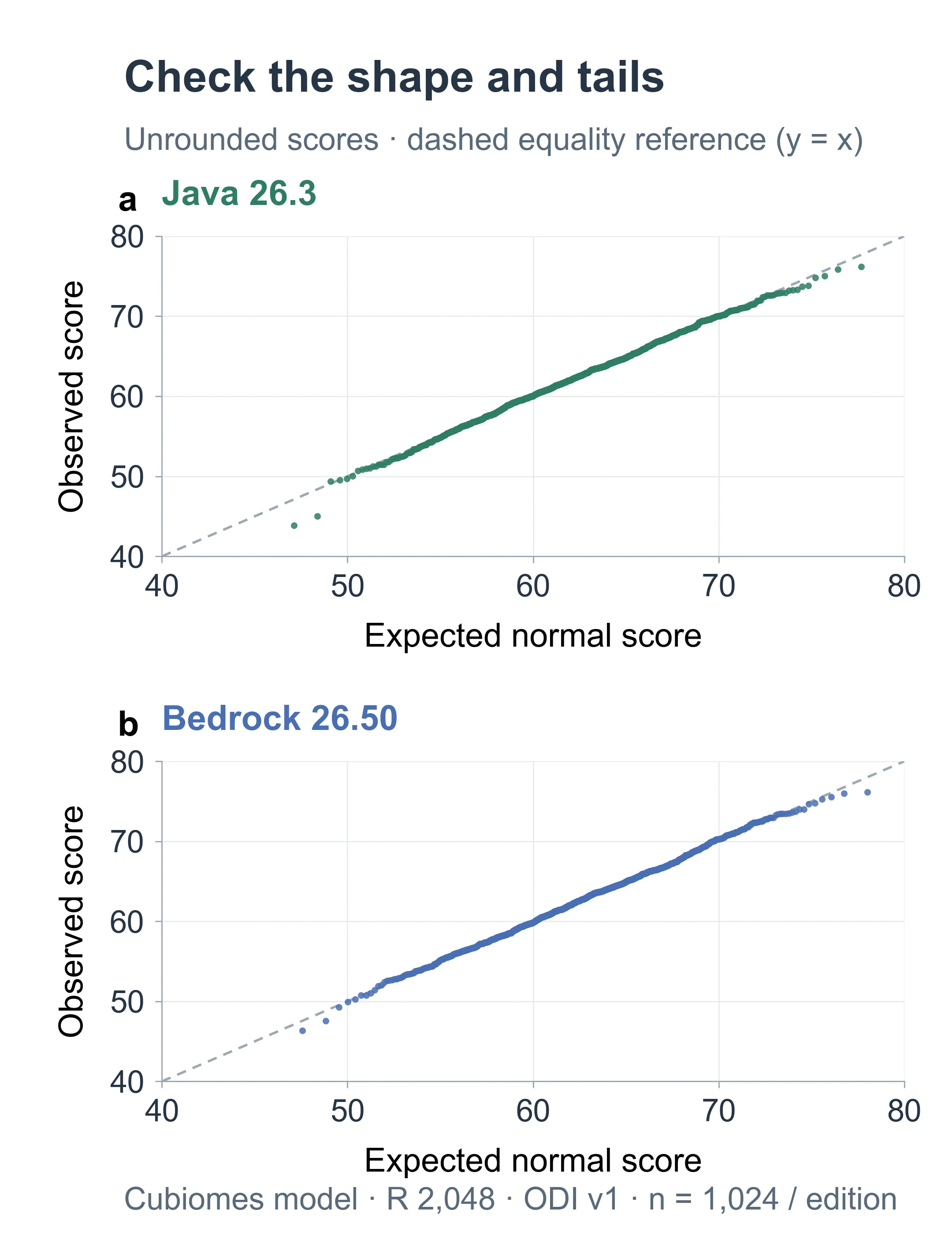
Each panel contains all 1,024 unrounded overall scores. Expected normal scores use the sample’s mean and standard deviation; the gray diagonal marks equal expected and observed values. It is not a confidence band.
Both axes use index points. A dot on the diagonal has the observed score expected at that position in the normal comparison. Dots above it have higher observed scores; dots below it have lower ones. The leftmost and rightmost dots represent the sample’s low and high tails.
Most points track the diagonal closely, with departures at the extremes. Those end points matter when the question concerns unusually low or high scores. A close fit through the center does not establish a reliable normal-curve estimate for a very rare score outside the observed range.
What the normality check establishes
We applied the Shapiro-Wilk test documented by SciPy to the unrounded overall score and both unrounded components in each edition. Using unrounded values avoids treating the display’s integer ties as continuous measurements. We used a threshold of 0.05 and Holm correction across those six tests.
| Tested distribution | Java 26.3 adjusted p-value | Bedrock 26.50 adjusted p-value | Result at 0.05 |
|---|---|---|---|
| Overall index | 0.667 | 0.667 | Departure not detected |
| Biome component | 0.0059 | 0.0059 | Departure detected |
| Structure component | 0.231 | 0.472 | Departure not detected |
The overall tests’ unadjusted p-values were 0.334 for Java and 0.660 for Bedrock. Their non-rejection is consistent with the approximate bell shapes in these particular samples. It does not prove normality, certify the generation models or tell us the probability that a world is enjoyable.
The scores remain bounded from 0 to 100. We use the actual observed frequencies for seed comparisons, without converting a score through a fitted normal curve. The tests and plots describe these two cohorts; other editions, versions, radii or future rubric revisions need their own evaluation.
The full statistical summary and all sampled model results retain the measurements behind these figures. The five distribution figures use the same paired sample; the distance-credit figure illustrates the formula.
Put an individual score in context
For the example seed Java 26.3 seed 12345, the calculator predicts a score of 69, with 30 of 35 families sampled and 14 of 17 structure types predicted. Those coverage counts amount to about 84 possible points before distance deductions: 50 × 30 / 35 + 50 × 14 / 17 ≈ 84. The nearest distances reduce that to the displayed 69. In the matching reference sample, 922 scores were lower, 27 were the same and 75 were higher.
The tied scores matter. Every displayed 69 represents a rounded result, and different combinations of biome credit and structure credit can produce it. The exact counts of lower, equal and higher displayed scores preserve those ties. They also explain the comparison more directly than silently assigning every tied seed the same estimated normal percentile.
The calculator shows the observed histogram, sample median, P10 to P90 range and counts below, equal to and above your score when the exact edition, version, radius, rubric and generation model match. Other settings still receive their discovery breakdown; they currently have no matched reference sample.
Encounter frequency also needs its own denominator. In the Java 26.3 cohort at this radius, the model sampled a mushroom-fields family in 294 of 1,024 seeds (28.7%) and predicted a woodland mansion in 158 (15.4%). These are occurrences somewhere inside the estimated-spawn circle, not the probability of spawning in that biome or a measure of its global area.
An overall-score histogram answers how often the calculator produced particular totals in this sample. A rarity-weighted criterion would ask a different question about the encounter frequency of particular families or structure types. Revision 1 keeps its equal weights within each category; these measurements have not been turned into rarity bonuses. Such a change would need encounter baselines matched to the edition, generation version, radius and sampling rules, plus a new reviewed rubric revision.
This is a reference sample of model predictions, not a population rarity percentile, a sample of played worlds or a measurement of how far players travel. A score of 80 does not mean a seed is more varied than 80% of all seeds. Use the calculator to compare the modeled discoveries in the area you intend to explore, then inspect the locations that matter to you on the seed map.